Two inevitabilities: Death and Churn
The core problem the KM estimator helps us deal with is missing data.
Cohort data is inherently flawed in that more recent cohorts have fewer data points to compare against older cohorts. For example, a five-month-old cohort can only be compared with the first five months of a ten-month-old cohort. The retention rates of a cohort of customers acquired seven months ago can only reasonably be compared to the first seven month retention of older cohorts.
Imagine you had the full retention history of the previous 12 monthly cohorts and you wanted to predict the 12-month retention curve of a newly acquired customer. It’s not at all obvious how to do this.
To understand this better, let’s visualize a simpler example with only five cohorts:
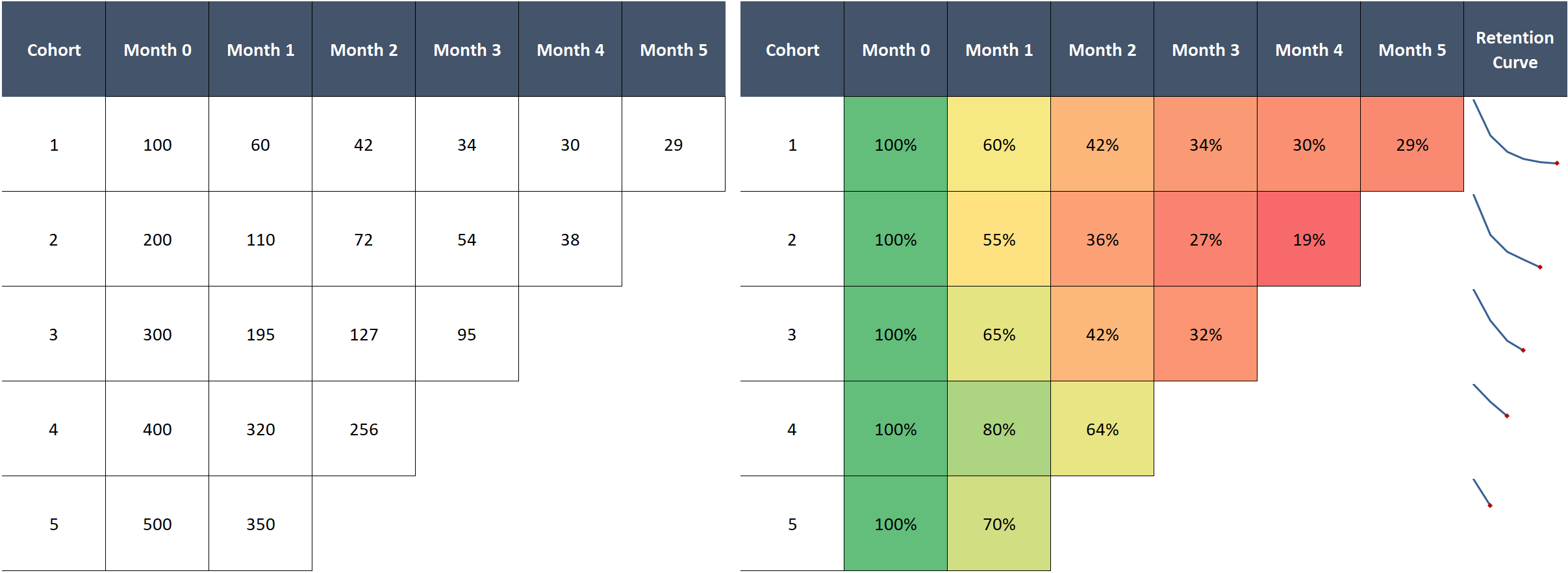
You might first try to calculate average retention across cohorts. This is problematic for two reasons:
- The simple average will not be representative if our cohorts differ in size
- For any given month we can only average over cohorts that have been alive at least that long, so we effectively average over fewer and fewer cohorts over time
We can see the second issue below. With both the simple and weighted average, we get strange results when performance oscillates across cohorts:
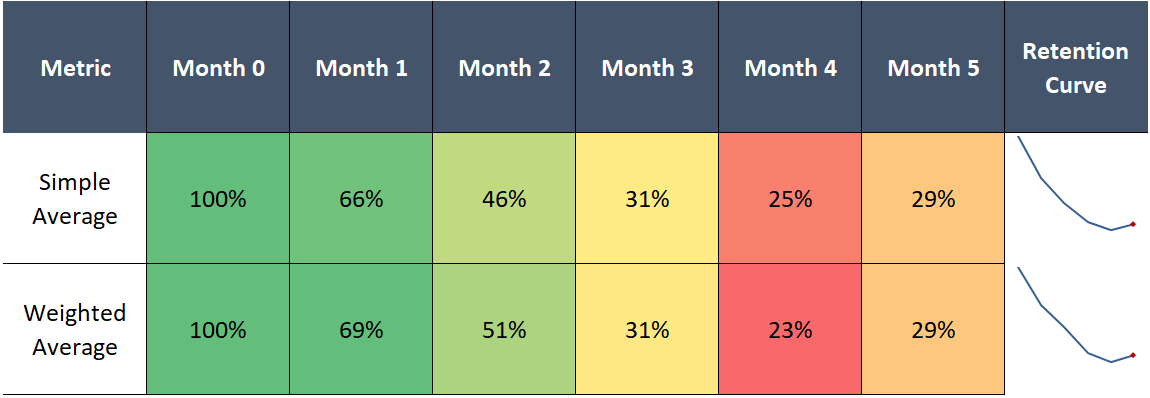
Assuming we don’t re-add returning users who previously churned into their original cohort, retention cannot possibly tick up after declining—it’s a one way street. This is an artifact of our flawed method, as 5-month retention cannot exceed 4-month retention by definition.
A third, related problem arises when comparing groups of cohorts to other groups, for example, comparing 2016’s group of monthly cohorts to 2017’s. As we’ve just shown, using averages to estimate retention curves for each group doesn’t work, which means we also cannot compare one group to another.
Questions? Ask your doctor

Believe it or not, clinical researchers deal with this same issue all the time.
Customer cohorts are analogous to groups of patients starting treatment at different times. Here the “treatment” is the time of customer acquisition and “death” is simply churn.
Or, imagine if the “2016 cohorts” and “2017 cohorts”, rather than being year-grouped cohorts, were groups receiving different treatments in a clinical trial. We want to quantify differences in patient survival rates (customer retention) between the two groups.
Pharmaceutical companies and other research outfits regularly contend with this. Patients start treatment at different times. Patients drop out of studies, by dying, but also by moving locations or deciding to stop taking the medication.
This creates a host of missing data issues at the beginning, middle, and end of any patient’s clinical test record, complicating analysis of effectiveness and safety.
To solve this problem, in 1958, a mathematician, Edward Kaplan, and statistician, Paul Meier, jointly created the Kaplan-Meier estimator. Also called the product-limit estimator, the method effectively deals with the missing data issue, providing a more precise estimate of the probability of survival up to any point.
The core idea behind Kaplan-Meier:
The estimated probability of surviving up to any point is the cumulative probability of surviving each preceding time interval, calculated as the product of the preceding survival probabilities
That strange formula above is simply multiplying a bunch of probabilities against one another to find the cumulative probability of survival at a certain point.
Where do these probabilities come from? Directly from the data.
KM says our best estimate of the probability of survival from one month to the next is exactly the weighted average retention rate for that month in our dataset (also called the maximum likelihood estimator in statistics parlance). So if in a group of cohorts we have 1000 customers from month one, of which 600 survive until month two, our best guess of the “true” probability of survival from month 1 to 2 is 60%.
We do the same for the next month. Divide the number of customers that survived through month 3 by the number of customers who survived through month 2 to get the estimated probability of survival from month 2 to 3. If we don’t have month 3 data for a cohort because it’s only two months old, we exclude those customers from our calculations for month 3 survival.
Repeat for as many cohorts / months as you have, excluding in each calculation any cohorts missing data for the current period. Then, to calculate the probability of survival through any given month, multiply the individual monthly (conditional) probabilities up through that month.
Though a morbid thought, measuring patient survival is functionally equivalent to measuring customer retention, so we can easily transfer KM to customer cohort analysis!
Putting Kaplan-Meier to the test
Let’s make this clearer by applying the Kaplan-Meier estimator to our previous example.
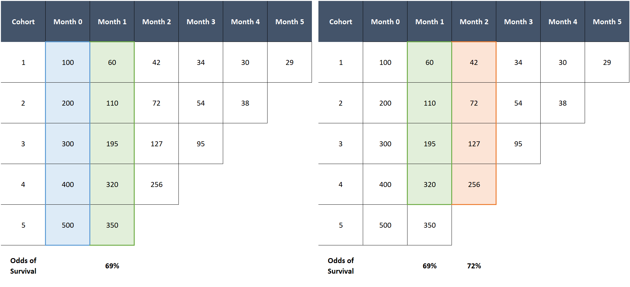
The probability of surviving month 1 is 69% (total customers alive in month 1 divided by total in month 0). The probability of surviving month 2, given a customer survived month 1, is 72% (total customers alive in month 2 divided by total in month 1, excluding the last cohort which is missing month 2 data). So the cumulative probability of surviving at least two months is 69% x 72% = 50%. Rinse, wash, and repeat for each subsequent month.
Side-by-side comparison reveals the superiority of KM:
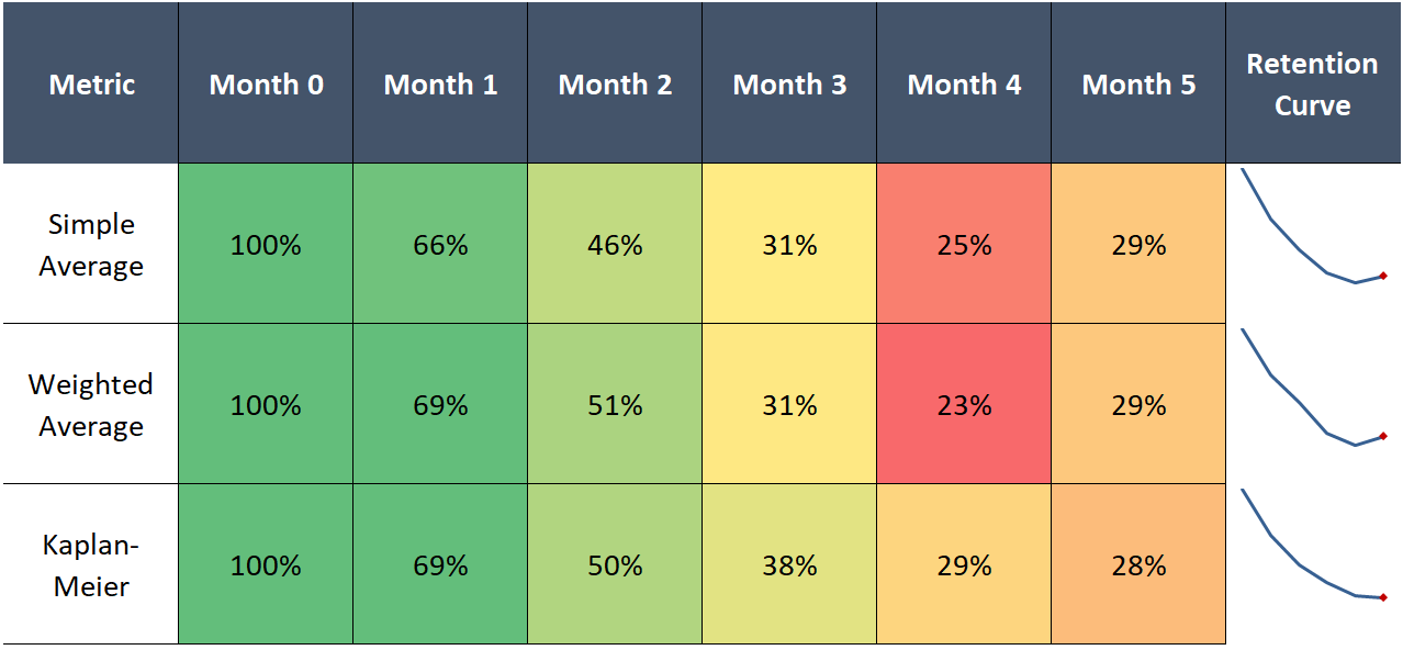
What’s great about KM is it leverages all the data we have, even the younger cohorts for whom we have fewer observations. For example, while the average of all the available cohorts at month 3 only uses the data for cohorts 1-3, due to its cumulative nature, the KM estimator effectively incorporates the improved early retention of the newer cohorts. This yields a 3-month retention estimate of 38%, which is higher than any of the cohorts we can actually measure at month 3.
This is exactly what we want—cohorts 4 and 5 are both larger and better retaining than 1-3. Hence, it is likely that the 3-month retention rate for a random customer picked among these cohorts will exceed the historical average, as the customer will likely be in cohorts 4 or 5.
Using all the data is also nice because it makes our estimates of the tail probabilities much more precise than if we could only rely on the data of customers who we retained that long.
Kaplan-Meier curves also fixes the wonky behavior in the right tail of the retention curve by respecting a fundamental law of probability: cumulative probabilities can only decline as you multiply more numbers.
Recommended by 95% of doctors
This analysis could easily be extended. Let’s go back to the 2016 vs 2017 example—we could run the Kaplan-Meier calculation on each respective group of cohorts and then compare the resulting survival curves, highlighting differences in expected retention between the two groups.
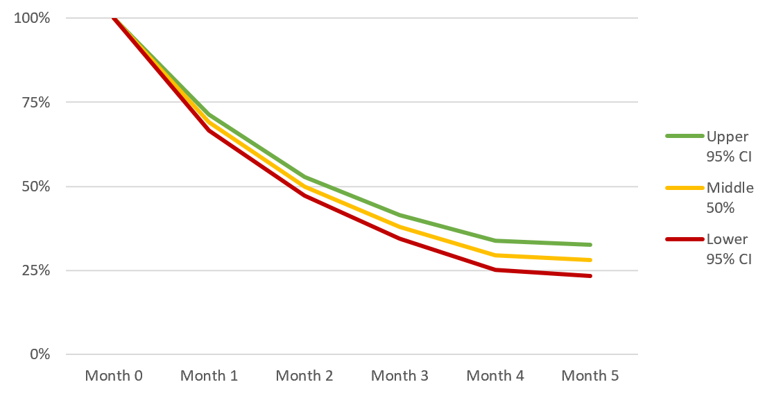
While I won’t cover it here, you can also calculate p-values, confidence intervals, and statistical significance tests for Kaplan-Meier curves. This lets you to make rigorous statements like “the improvement of cohort retention in 2018 relative to 2017 was statistically significant (at the 5% level)”—cool stuff:
Kaplan-Meier is a powerful tool for anyone who spends time analyzing customer cohort data. KM has been battle-tested in rigorous clinical trials—if anything it’s surprising it hasn’t caught on more among technology operators and investors.
If you're a product manager, growth hacker, marketer, data scientist, investor, or anyone else who understands the deep importance of customer retention analysis, the Kaplan-Meier estimator should be a valuable weapon in your analytics arsenal.